Intro to Grids

A basic introduction to the GridSpectra class.

import numpy as np
import matplotlib.pyplot as plt

from GridPolator import GridSpectra

Let’s create our own grid

Let’s think of something that can be created programically but it also simple to visualize. Imagine the class of functions:

\[y = a x (x-b)\]

There are two parameters, \(a\) and \(b\), and the graph always passes through the origin.

Suppose we want to know the value of this function with \(a ~ [-3,3]\) and \(b ~[-5,5]\). Suppose also that each “spectrum” has some expensive physics in it, so we don’t want to calculate too many, but a high resolution in \(x\) is okay.

a = np.linspace(-3, 3, 7)
b = np.linspace(-5, 5, 9)
x = np.linspace(1, 10, 1000)

spec = np.zeros(shape=(len(a), len(b), len(x)))

for i,_a in enumerate(a):
    for j,_b in enumerate(b):
        _s = _a * x * (x - _b)
        spec[i, j, :] = _s

Initialize the interpolator

We now pass all of this information to the GridSpectra class.

g = GridSpectra(
    native_wl=x,
    params={
        'a': a,
        'b': b
    },
    spectra=spec,
    impl='scipy' # or 'jax', see docs for more
)

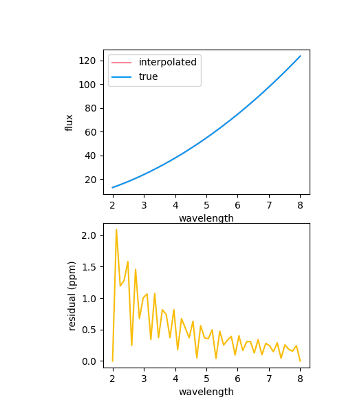
Evaluate

We pass the interpolator a new wavelength grid along with new parameters and it will interpolate to give us a new spectrum.

new_wl = np.linspace(2,8,50)
__a = 1.5
__b = -2.3
new_spec = g.evaluate(
    (
        np.array([__a]),
        np.array([__b])
        ),
    new_wl
)[0]
true_spec = __a * new_wl * (new_wl - __b)

fig,axes = plt.subplots(2,1,figsize=(5,6))
ax = axes[0]
rax = axes[1]
fig.subplots_adjust(left=0.3)
ax.plot(new_wl, new_spec, label='interpolated',c='xkcd:rose pink')
ax.plot(new_wl, true_spec, label='true',c='xkcd:azure')
rax.plot(new_wl, (new_spec - true_spec)/true_spec*1e6, label='difference (ppm)',c='xkcd:golden rod')
ax.set_xlabel('wavelength')
rax.set_xlabel('wavelength')
ax.set_ylabel('flux')
rax.set_ylabel('residual (ppm)')
_=ax.legend()